yam Documentation

Motivation

Why another monitoring tool for seismic velocities using ambient noise cross-correlations?

There are several alternatives around, namely MSNoise and MICC MIIC. MSNoise is especially useful for large datasets and continuous monitoring. Configuration and the state of a project is managed by sqlite or mysql database. A project can be configured via web interface, commands are issued via command line interface. Velocity variations are determined with the Moving Window Cross Spectral technique (MWCS). MIIC is another monitoring library using the time-domain stretching technique.

Yam, contrary to MSNoise, is designed to work with completed datasets, but also includes capabilities to process new additional data. Yam does not rely onto a database, but rather checks on the fly which results already exist and which results have still to be calculated. Cross-correlations are written to HDF5 files via the ObsPy plugin obspyh5. Thus, correlation data can be easily accessed with ObsPy’s read() function after the calculation. It follows a similar processing flow as MSNoise, but it uses the stretching similar to MIIC. (It is of course feasible to implement MWCS.) One of its strong points is the configuration declared in a simple, but heavily commented JSON file. It is possible to declare similar configurations. A possible use case is the reprocessing of the whole dataset in a different frequency band. Some code was reused from previous project sito.

Installation

Dependencies of yam are obspy>=1.1 obspyh5>=0.3 h5py tqdm. Optional dependencies are IPython and cartopy. The recommended way to install yam is via anaconda and pip:

conda --add channels conda-forge
conda create -n yam cartopy h5py IPython obspy tqdm
conda activate yam
pip install yam

After that, you can run the tests with yam-runtests and check if everything is installed properly.

How to use yam

The scripts are started with the command line program yam. yam -h gives an overview over available commands and options. Each command has its own help, e.g. yam correlate -h will print help for the correlate command.

create will create an example configuration file in JSON format. The processing commands correlate, stack and stretch support parallelization. The number of cores can be specified with the --njobs flag, by default all available cores are used.

info, print, load and plot commands allow to inspect correlations, stacks and stretching results as well as preprocessed data and other aspects. remove removes correlations or stretching results (necessary if configuration changed).

Correlations, corresponding stacks and stretching results are saved in HDF5 files. The indices inside the HDF5 files are the following (first for correlations, second for stretching results):

'{key}/{network1}.{station1}-{network2}.{station2}/{location1}.{channel1}-{location2}.{channel2}/{starttime.year}-{starttime.month:02d}/{starttime.datetime:%Y-%m-%dT%H:%M}'
'{key}/{network1}.{station1}-{network2}.{station2}/{location1}.{channel1}-{location2}.{channel2}'

The strings are expanded with the corresponding metadata. Several tools are available for analysing the contents of the HDF5 files, e.g. h5ls or hdfview.

About keys and different configurations

key in the above indices and as a parameter in the command line interface is a special parameter which describes the processing chain. It is best explained with an example: A key could be c1_s2d_twow. This means data was correlated (c) with configuration 1, each two days 2d are stacked (s) and finally data was stretched (t) using the stretching configuration wow. The configuration of the keys are defined in the configuration file. (These ids may not contain _, because _ is used to separate the different processing steps.) The s key is special, because it can describe the stacking procedure directly: For example, s5d stacks correlations of 5 days, s2h of 2 hours, s5dm2.5d is a 2.5 day moving (m) stack over 5 days, with d corresponding to days and h corresponding to hours. But s can also precede a key which is described in the configuration file.

Valid processing chains could be represented by c2 (data is only correlated), c2_t2 (and directly stretched afterwards), c1_s10dm5d_t1 (correlation, moving stack, stretch), c1_s1d_s5dm2d (correlation, stack, moving stack) or similar.

Tutorial

A small tutorial with an example dataset is included. It can be loaded into an empty directory with yam create --tutorial. Plots are created in a separate plots folder and can be interactively shown with the --show flag. Please open a console to work through the example command sequence. It is recommended to open the configuration file to simultaneously check the configuration of the keys used:

mkdir yam_tutorial; cd yam_tutorial  # switch to empty directory
yam create --tutorial  # load tutorial dataset and configuration file

yam info               # plot information about project
yam info stations      # print inventory info
yam info data          # plot info about data files
yam plot stations      # plot station map (needs cartopy)
yam print data CX.PATCX..BHZ 2010-02-03       # load data for a specific station and day and print information
yam load data CX.PATCX..BHZ 2010-02-03        # load data for a specific station and day and start an IPython session
yam plot data CX.PATCX..BHZ 2010-02-03        # plot a day file
yam plot prepdata CX.PATCX..BHZ 2010-02-03 1  # plot the preprocessed data of the same day
                                              # (preprocessing defined in corr config 1)
yam correlate 1        # correlates data with corr configuration 1
yam correlate 1        # should finish fast, because everything is already calculated
yam correlate auto     # correlate data with another configuration suitable for auto-correlations
yam plot c1_s1d --plottype vs_dist  # plot correlation versus distance
yam plot cauto --plot-options '{"xlim": [0, 10]}'  # plot auto-correlations versus time and change some options
                                                   # ("wiggle" plot also possible)
yam stack c1_s1d 3dm1d       # stack 1 day correlations with a moving stack of 3 days
yam stack cauto 2            # stack auto-correlations with stack configuration 2

yam stretch c1_s1d_s3dm1d 1  # stretch the stacked data with stretch configuration 1
yam stretch cauto_s2 2       # stretch the stacked auto-correlations with another stretch configuration
yam info                     # find out about the keys which are already in use
yam plot cauto_s2_t2         # plot similarity matrices for the given processing chain
yam plot cauto_s2_t2 --plot-options '{"show_line": true}' --show  # plot similarity matrices and show
                                                                  # an interactive plot
yam plot c1_s1d_s3dm1d_t1/CX.PATCX-CX.PB01  # plot similarity matrices, but only for one station combination
                                            # (restricting the group is also possible for stacking and stretching)

Of course, the plots do not look overwhelmingly for such a small dataset.

Two advanced tutorials are available as Jupyter notebooks:

• Inter-station cross-correlations

• Monitoring seismic velocity

Further resources are listed in the readme of the Github repository.

Use your own data

Create the example configuration with yam create and adapt it to your needs. A good start is to change the inventory and data parameters.

Read correlation and results of stretching procedure in Python for further processing

Use ObsPy’s read() to read correlations and stacks and read_dicts() to read stretching results.

from obspy import read
from yam import read_dicts

# read a whole file of correlations
stream = read('corr.h5', 'H5')
# to read only part of a file
stream = read('stack.h5', 'H5', include_only=dict(key='c1_s1d', network1='CX', station1='PATCX',
                                                  network2='CX', station2='PB01'))
# or specify the group explicitly
stream = read('stack.h5', 'H5', group='c1_s1d')
# read the stretching results into a dictionary
stretch_result = read_dicts('stretch.h5', 'c1_s1d_t1')

Configuration options

Please see the example configuration file configuration file for an explanation of configuration options. It follows a table with links to functions which consume the options. All config options should be documented inside these functions.

configuration dictionary	functions consuming the options
io	Configuration for input and output (needed by most functions in commands module)
correlate	start_correlate -> correlate -> preprocess -> time_norm, spectral_whitening
stack	start_stack -> _stack_wrapper -> stack
stretch	start_stretch -> _stretch_wrapper -> stretch
plot_*_options	See corresponding functions in imaging module

More information about the different subcommands of yam can be found in the corresponding functions in commands module.

API Documentation

Yam consists of the following modules:

correlate	Preprocessing and correlation
stack	Stack correlations
stretch	Stretch correlations
imaging	Plotting functions
main	Command line interface and main entry point
commands	Commands used by the CLI interface
util	Utility functions

correlate Module

Preprocessing and correlation

yam.correlate.correlate(io, day, outkey, edge=60, length=3600, overlap=1800, demean_window=True, discard=None, only_auto_correlation=False, station_combinations=None, component_combinations=('ZZ',), max_lag=100, keep_correlations=False, stack='1d', njobs=0, **preprocessing_kwargs)

Correlate data of one day

Parameters:

• io – io config dictionary

• day – UTCDateTime object with day

• outkey – the output key for the HDF5 index

• edge – additional time span requested from day before and after in seconds

• length – length of correlation in seconds (string possible)

• overlap – length of overlap in seconds (string possible)

• demean_window – demean each window individually before correlating

• discard – discard correlations with less data coverage (float from interval [0, 1])

• only_auto_correlations – Only correlate stations with itself (different components possible)

• station_combinations – specify station combinations (e.g. 'CX.PATCX-CX.PB01, network code can be omitted, e.g. 'PATCX-PB01', default: all)

• component_combinations – component combinations to calculate, tuple of strings with length two, e.g. ('ZZ', 'ZN', 'RR'), if 'R' or 'T' is specified, components will be rotated after preprocessing, default: only ZZ components

• max_lag – max time lag in correlations in seconds

• keep_correlatons – write correlations into HDF5 file (dafault: False)

• stack –

  stack correlations and write stacks into HDF5 file (default: '1d', must be smaller than one day or one day)

  Note

  If you want to stack larger time spans use the separate stack command on correlations or stacked correlations.

• njobs – number of jobs used. Some tasks will run parallel (preprocessing and correlation).

• **preprocessing_kwargs – all other kwargs are passed to preprocess

yam.correlate.correlate_traces(tr1, tr2, maxshift=3600, demean=True)

Return trace of cross-correlation of two input traces

Parameters:

• tr1,tr2 – two Trace objects

• maxsift – maximal shift in correlation in seconds

yam.correlate.get_data(smeta, data, data_format, day, overlap=0, edge=0, trim_and_merge=False)

Return data of one day

Parameters:

• smeta – dictionary with station metadata

• data – string with expression of data day files or function that returns the data (aka get_waveforms)

• data_format – format of data

• day – day as UTCDateTime object

• overlap – overlap to next day in seconds

• edge – additional time span requested from day before and after in seconds

• trim_and_merge – wether data is trimmed to day boundaries and merged

yam.correlate.preprocess(stream, day=None, inventory=None, overlap=0, remove_response=False, remove_response_options=None, demean=True, filter=None, normalization=(), time_norm_options=None, spectral_whitening_options=None, downsample=None, tolerance_shift=None, interpolate_options=None, decimate=None, njobs=0)

Preprocess stream of 1 day

Parameters:

• stream – Stream object

• day – UTCDateTime object of day (for trimming)

• inventory – Inventory object (for response removal)

• remove_response (bool) – remove response

• filter – min and max frequency of bandpass filter

• normalizaton – ordered list of normalizations to apply, 'sprectal_whitening' for spectral_whitening and/or one or several of the time normalizations listed in time_norm

• downsample – downsample before preprocessing, target sampling rate

• tolerance_shift – Samples are aligned at “good” times for the target sampling rate. Specify tolerance in seconds. (default: no tolerance)

• decimate – decimate further by given factor after preprocessing (see Trace.decimate)

• njobs – number of parallel workers

• *_options – dictionary of options passed to the corresponding functions

yam.correlate.spectral_whitening(tr, smooth=None, filter=None, waterlevel=1e-08, mask_again=True)

Apply spectral whitening to data

Data is divided by its smoothed (Default: None) amplitude spectrum.

Parameters:

• tr – trace to manipulate

• smooth – length of smoothing window in Hz (default None -> no smoothing)

• filter – filter spectrum with bandpass after whitening (tuple with min and max frequency)

• waterlevel – waterlevel relative to mean of spectrum

• mask_again – wether to mask array after this operation again and set the corresponding data to 0

Returns:

whitened data

yam.correlate.time_norm(tr, method, clip_factor=None, clip_set_zero=None, clip_value=2, clip_std=True, clip_mode='clip', mute_parts=48, mute_factor=2, plugin=None, plugin_options={})

Calculate normalized data, see e.g. Bensen et al. (2007)

Parameters:

• tr – Trace to manipulate

• method (str) –

  1bit: reduce data to +1 if >0 and -1 if <0

  clip: clip data to value or multiple of root mean square (rms)

  mute_envelope: calculate envelope and set data to zero where envelope is larger than specified plugin: use own function

• mask_zeros – mask values that are set to zero, they will stay zero in the further processing

• clip_value (float) – value for clipping or list of lower and upper value

• clip_std (bool) – Multiply clip_value with rms of data

• clip_mode (bool) – ‘clip’: clip data ‘zero’: set clipped data to zero ‘mask’: set clipped data to zero and mask it

• mute_parts (int) – mean of the envelope is calculated by dividing the envelope into several parts, the mean calculated in each part and the median of this averages defines the mean envelope

• mute_factor (float) – mean of envelope multiplied by this factor defines the level for muting

• plugin (str) – function in the form module:func

• plugin_options (dict) – kwargs passed to plugin

Returns:

normalized data

stack Module

Stack correlations

yam.stack.stack(stream, length=None, move=None)

Stack traces in stream by correlation id

Parameters:

• stream – Stream object with correlations

• length – time span of one trace in the stack in seconds (alternatively a string consisting of a number and a unit – 'd' for days and 'h' for hours – can be specified, i.e. '3d' stacks together all traces inside a three days time window, default: None, which stacks together all traces)

• move – define a moving stack, float or string, default: None – no moving stack, if specified move usually is smaller than length to get an overlap in the stacked traces

Returns:

Stream object with stacked correlations

stretch Module

Stretch correlations

The results are returned in a dictionary with the following entries:

times:

strings of starttimes of the traces (1D array, length N1)

velchange_values:

velocity changes (%) corresponding to the used stretching factors (assuming a homogeneous velocity change, 1D array, length N2)

tw:

used lag time window

sim_mat:

similarity matrices (2D array, dimension (N1, N2))

velchange_vs_time:

velocity changes (%) as a function of time (value of highest correlation/similarity for each time, length N1)

corr_vs_time:

correlation values as a function of time (value of highest correlation/similarity for each time, length N1)

attrs:

dictionary with metadata (e.g. network, station, channel information of both stations, inter-station distance and parameters passed to the stretching function)

yam.stretch.average_dicts(dicts)

Average list of dictionaries with stretching results

yam.stretch.join_dicts(dicts)

Join list of dictionaries with stretching results

yam.stretch.stretch(stream, max_stretch, num_stretch, tw, tw_relative=None, reftr=None, sides='both', max_lag=None, time_period=None)

Stretch traces in stream and return dictionary with results

See e.g. Richter et al. (2015) for a description of the procedure.

Parameters:

• stream – Stream object with correlations

• max_stretch (float) – stretching range in percent

• num_stretch (int) – number of values in stretching vector

• tw – definition of the time window in the correlation – tuple of length 2 with start and end time in seconds (positive)

• tw_relative – time windows can be defined relative to a velocity, default None or 0 – time windows relative to zero lag time, otherwise velocity is given in km/s

• reftr – reference trace, by default the stack of stream is used as reference

• sides – one of left, right, both

• max_lag – max lag time in seconds, stream is trimmed to (-max_lag, max_lag) before stretching

• time_period – use correlations only from this time span (tuple of dates)

imaging Module

Plotting functions

Common arguments in plotting functions are:

stream:

Stream object with correlations

fname:

file name for the plot output

ext:

file name extension (e.g. 'png', 'pdf')

figsize:

figure size (tuple of inches)

dpi:

resolution of image file (not available for station plot)

xlim:

limits of x axis (tuple of lag times or tuple of UTC strings)

ylim:

limits of y axis (tuple of UTC strings or tuple of percentages)

*_kw:

dictionary of arguments passed to calls of matplotlib methods (e.g. plot_kw for arguments passed to Axes.plot(), etc). Some of these dictionaries might be set to None to suppress the corresponding feature (e.g. set stack_plot_kw=None to not plot the stack of all traces in plot_corr_vs_time()).

yam.imaging.plot_corr_vs_dist(stream, fname=None, figsize=(10, 5), ext='png', dpi=None, components='ZZ', scale=1, dist_unit='km', xlim=None, ylim=None, time_period=None, plot_kw={})

Plot stacked correlations versus inter-station distance

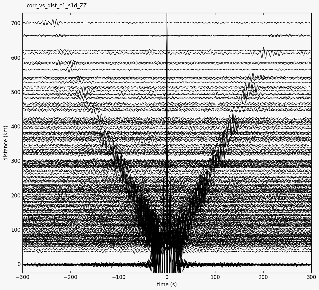
This plot can be created from the command line with --plottype vs_dist.

Parameters:

• components – component combination to plot

• scale – scale wiggles (default 1)

• dist_unit – one of ('km', 'm', 'deg')

Time_period:

use correlations only from this time span (tuple of dates)

yam.imaging.plot_corr_vs_time(stream, fname=None, figsize=(10, 5), ext='png', dpi=None, xlim=None, ylim=None, vmax=None, cmap='RdBu_r', stack_plot_kw={})

Plot correlations versus time

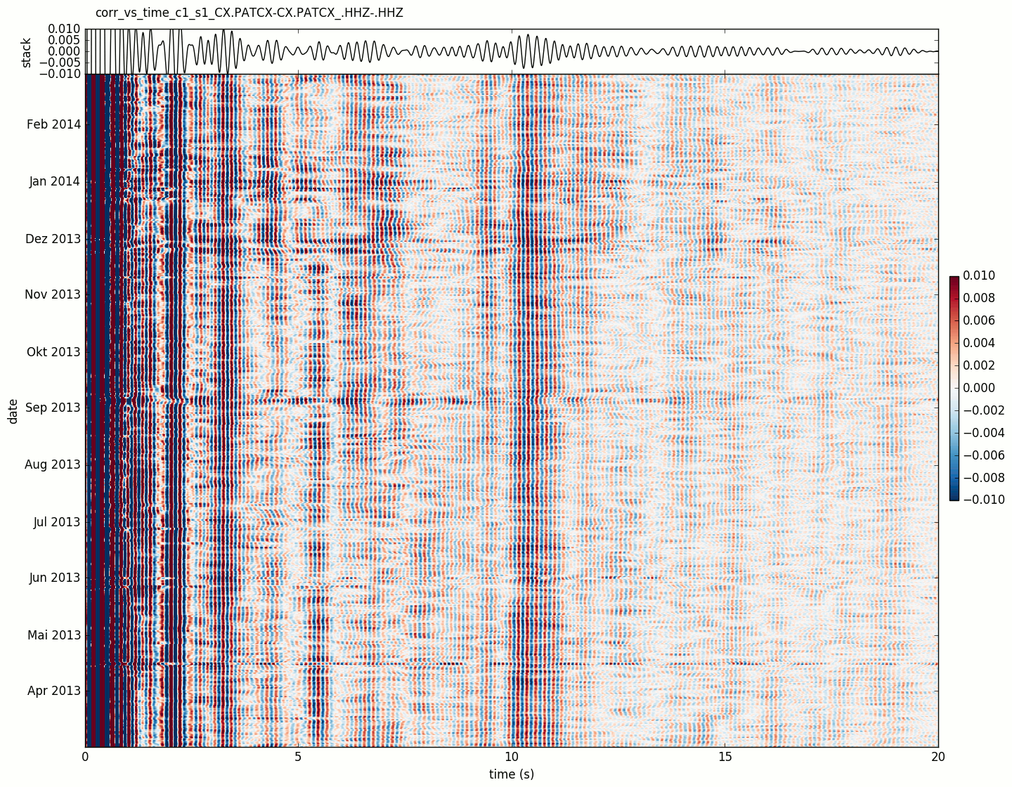
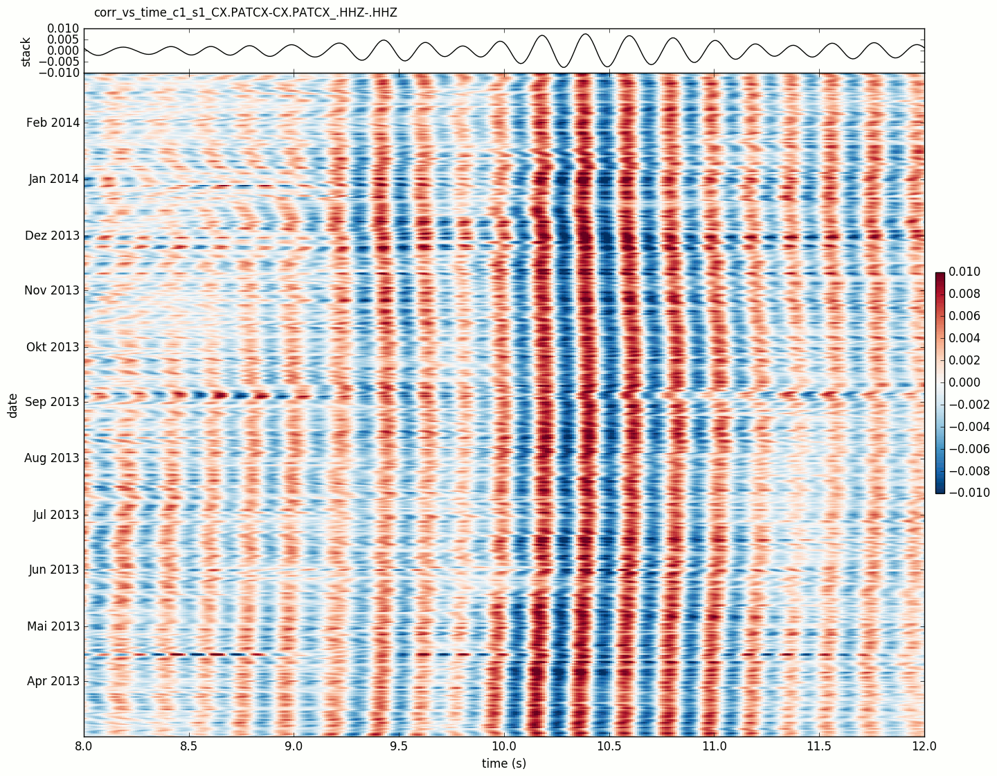
Default correlation plot.

Parameters:

• vmax – maximum value in colormap

• cmap – used colormap

yam.imaging.plot_corr_vs_time_wiggle(stream, fname=None, figsize=(10, 5), ext='png', dpi=None, xlim=None, ylim=None, scale=20, plot_kw={})

Plot correlation wiggles versus time

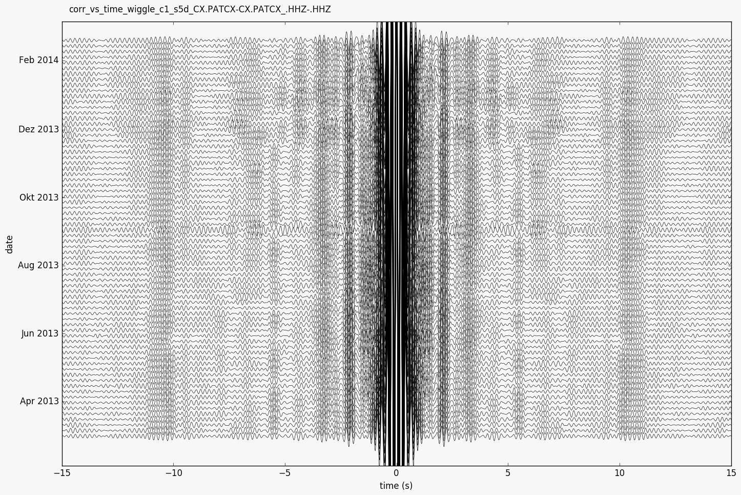
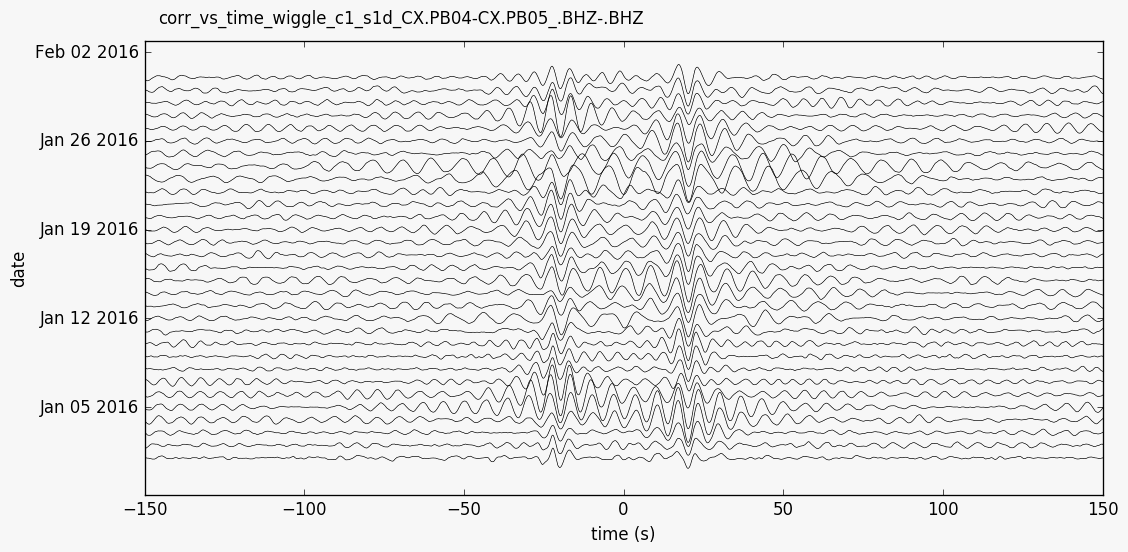
This plot can be created from the command line with --plottype wiggle.

Parameters:

scale – scale of wiggles (default 20)

yam.imaging.plot_data(data, fname, ext='png', show=False, type='dayplot', **kwargs)

Plot data (typically one day)

Parameters:

• data – Stream object holding the data

• type,**kwargs – passed to Stream.plot() method

yam.imaging.plot_sim_mat(res, fname=None, figsize=(10, 5), ext='png', dpi=None, xlim=None, ylim=None, vmax=None, cmap='hot_r', show_line=False, line_plot_kw={})

Plot similarity matrices

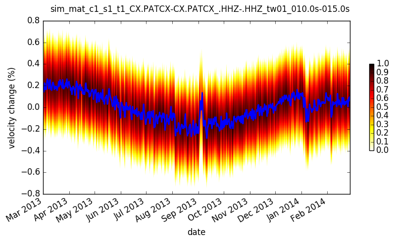
Default plot for stretching results.

Parameters:

• res – dictionary with stretching results

• vmax – maximum value in colormap

• cmap – used colormap

• show_line – show line connecting best correlations for each time

yam.imaging.plot_stations(inventory, fname, ext='png', projection='local', **kwargs)

Plot station map

Parameters:

• inventory – Inventory object with coordinates

• projection,**kwargs – passed to Inventory.plot() method

yam.imaging.plot_velocity_change(results, fname=None, figsize=(10, 5), ext='png', dpi=None, xlim=None, ylim=None, plot_kw={}, joint_plot_kw={}, legend_kw={})

Plot velocity change over time

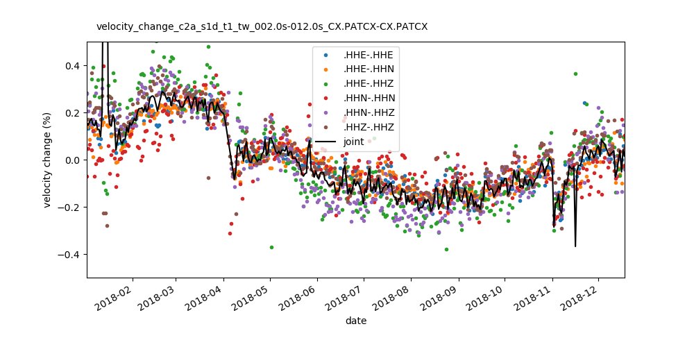
Plot velocity change over time estimated from different component/station combinations and joint estimate. This plot can be created from the command line with --plottype velocity.

Parameters:

results – list of dictionaries with stretching results

main Module

Command line interface and main entry point

class yam.main.ConfigJSONDecoder(*, object_hook=None, parse_float=None, parse_int=None, parse_constant=None, strict=True, object_pairs_hook=None)

decode(s)

Decode JSON config with comments stripped

yam.main.run(command, conf=None, tutorial=False, less_data=False, pdb=False, **args)

Main entry point for a direct call from Python

Example usage:

>>> from yam import run
>>> run(conf='conf.json')

Parameters:

command – if 'create' the example configuration is created, optionally the tutorial data files are downloaded

For all other commands this function loads the configuration and construct the arguments which are passed to run2()

All args correspond to the respective command line and configuration options. See the example configuration file for help and possible arguments. Options in args can overwrite the configuration from the file. E.g. run(conf='conf.json', bla='bla') will set bla configuration value to 'bla'.

yam.main.run2(command, io, logging=None, verbose=0, loglevel=3, logfile=None, key=None, keys=None, corrid=None, stackid=None, stretchid=None, correlate=None, stack=None, stretch=None, **args)

Second main function for unpacking arguments

Initialize logging, load inventory if necessary, load options from configuration dictionary into args (for correlate, stack and stretch commands) and run the corresponding command in commands module. If "based_on" key is set the configuration dictionary will be preloaded with the specified configuration.

Parameters:

• command – specified subcommand, will call one of start_correlate(), start_stack(), start_stretch(), info(), load(), plot(), remove()

• logging,verbose,loglevel,logfile – logging configuration

• key – the key to work with

• keys – keys to remove (only remove command)

• correlate,stack,stretch – corresponding configuration dictionaries

• *id – the configuration id to load from the config dictionaries

• **args – all other arguments are passed to next called function

yam.main.run_cmdline(args=None)

Main entry point from the command line

commands Module

Commands used by the CLI interface

yam.commands._stack_wrapper(groupnames, fname, outkey, **kwargs)

Wrapper around stack()

Parameters:

• groupnames – groups to load the correlations from

• fname – file to load correlations from

• outkey – key to write stacked correlations to

• **kwargs – all other kwargs are passed to stack() function

yam.commands._stretch_wrapper(groupnames, fname, outkey, filter=None, **kwargs)

Wrapper around stretch()

Parameters:

• groupname – group to load the correlations from

• fname – file to load correlations from

• fname_stretch – file for writing results

• outkey – key to write stretch results to

• filter – filter correlations before stretching (bandpass, tuple with min and max frequency)

• **kwargs – all other kwargs are passed to stretch() function

yam.commands.info(io, key=None, subkey='', config=None, **unused_kwargs)

Print information about yam project

Parameters:

• io – io configuration dictionary

• key – key to print infos about (key inside HDF5 file, or one of data, stations, default: None – print overview)

• subkey – only print part of the HDF5 file

• config – list of configuration dictionaries

yam.commands.load(io, key, seedid=None, day=None, do='return', prep_kw={}, fname=None, format=None)

Load object and do something with it

Parameters:

• io – io

• key – key of object to load (key inside HDF5 file, or one of data, prepdata, stations)

• seedid – seed id of a channel (for data or prepdata)

• day – UTCDateTime object with day (for data or prepdata)

• do – specifies what to do with the object, default is 'return' which simply returns the object, other possible values are 'print' – print object (used by print command), 'load' – load object in IPython session (used by load command), 'export' – export correlations to different file format (used by export command)

• prep_kw (dict) – options passed to preprocess (for prepdata only)

• fname – file name (for export command)

• format – target format (for export command)

yam.commands.plot(io, key, plottype=None, seedid=None, day=None, prep_kw={}, corrid=None, show=False, **kwargs)

Plot everything

Parameters:

• io – io configuration dictionary

• key – key of objects to plot, or one of stations, data, prepdata

• plottype – plot type to use (non default values are 'vs_dist' and 'wiggle' for correlation plots, 'velocity' for plots of stretching results)

• seedid – seed id of a channel (for data or prepdata)

• day – UTCDateTime object with day (for data or prepdata)

• prep_kw (dict) – options passed to preprocess (for prepdata only)

• corrid – correlation configuration (for prepdata only)

• show – show interactive plot

• **kwargs – all other kwargs are passed to the corresponding plot function in imaging module

yam.commands.remove(io, keys)

Remove one or several keys from HDF5 file

Parameters:

• io – io configuration dictionary

• keys – list of keys to remove

yam.commands.start_correlate(io, filter_inventory=None, startdate='1990-01-01', enddate='2020-01-01', njobs=None, parallel_inner_loop=False, keep_correlations=False, stack='1d', dataset_kwargs=None, **kwargs)

Start correlation

Parameters:

• io – io configuration dictionary

• filter_inventory – filter inventory with its select method, specified dict is passed to Inventory.filter()

• startdate,enddate (str) – start and end date as strings

• njobs – number of cores to use for computation, days are computed parallel, this might consume much memory, default: None – use all available cores, set njobs to 0 for sequential processing

• parallel_inner_loop – Run inner loops parallel instead of outer loop (preproccessing of different stations and correlation of different pairs versus processing of different days). Useful for a datset with many stations.

• dtype – data type for storing correlations (default: float16 - half precision)

• dataset_kwargs – options passed to obspyh5 resp. h5py when creating a new dataset, e.g. dataset_kwargs={'compression':'gzip'}. See create_dataset in h5py for more options. By default the dtype is set to 'float16'.

• keep_correlations,stack,**kwargs – all other kwargs are passed to correlate() function

yam.commands.start_stack(io, key, outkey, subkey='', njobs=None, starttime=None, endtime=None, dataset_kwargs=None, **kwargs)

Start stacking

Parameters:

• io – io configuration dictionary

• key – key to load correlations from

• outkey – key to write stacked correlations to

• subkey – only use a part of the correlations

• njobs – number of cores to use for computation, default: None – use all available cores, set njobs to 0 for sequential processing

• starttime,endtime – constrain start and end dates

• dataset_kwargs – options passed to obspyh5 resp. h5py when creating a new dataset, e.g. dataset_kwargs={'compression':'gzip'}. See create_dataset in h5py for more options. By default the dtype is set to 'float16'.

• **kwargs – all other kwargs are passed to yam.stack.stack() function

yam.commands.start_stretch(io, key, subkey='', njobs=None, reftrid=None, starttime=None, endtime=None, dataset_kwargs=None, **kwargs)

Start stretching

Parameters:

• io – io configuration dictionary

• key – key to load correlations from

• subkey – only use a part of the correlations

• njobs – number of cores to use for computation, default: None – use all available cores, set njobs to 0 for sequential processing

• reftrid – Parallel processing is only possible when this parameter is specified. Key to load the reference trace from, e.g. 'c1_s', it can be created by a command similar to yam stack c1 ''.

• starttime,endtime – constrain start and end dates

• dataset_kwargs – options passed to obspyh5 resp. h5py when creating a new dataset, e.g. dataset_kwargs={'compression':'gzip'}. See create_dataset in h5py for more options. By default the dtype is set to 'float16'.

• **kwargs – all other kwargs are passed to _stretch_wrapper() function

util Module

Utility functions

exception yam.util.ConfigError

class yam.util.IterTime(startdate, enddate, dt=86400)

Iterator yielding UTCDateTime objects between start- and endtime

exception yam.util.ParseError

class yam.util.TqdmLoggingHandler(level=0)

emit(record)

Do whatever it takes to actually log the specified logging record.

This version is intended to be implemented by subclasses and so raises a NotImplementedError.

exception yam.util.YamError

yam.util.create_config(conf='conf.json', tutorial=False, less_data=False)

Create JSON config file and download tutorial data if requested

yam.util.smooth(x, window_len=None, window='flat', method='zeros')

Smooth the data using a window with requested size.

This method is based on the convolution of a scaled window with the signal.

Parameters:

• x – the input signal (numpy array)

• window_len – the dimension of the smoothing window; should be an odd integer

• window – the type of window from ‘flat’, ‘hanning’, ‘hamming’, ‘bartlett’, ‘blackman’ flat window will produce a moving average smoothing.

• method –

  handling of border effects

  ’zeros’: zero padding on both ends (len(smooth(x)) = len(x))

  ’reflect’: pad reflected signal on both ends (same)

  ’clip’: pad signal on both ends with the last valid value (same)

  None: no handling of border effects (len(smooth(x)) = len(x) - len(window_len) + 1)

Example Configuration File

### Configuration file for yam package in json format
# Comments are indicated with "#" and ignored while parsing

{


### Logging options

# Loglevels 3=debug, 2=info, 1=warning, 0=error and log file
# Verbosity can be set on the command line or here

#"verbose": 3,
"loglevel": 3,
"logfile": "yam.log",



### Options for input and output

"io": {
        # Glob expression of station inventories
        "inventory": "example_inventory/CX.*.xml",

        # Expression for data file names (each 1 day). It will be evaluated by
        # string.format(t=day_as_utcdatetime, **station_meta).
        # The default value corresponds to the default naming of ObsPys FDSN Massdownloader.
        # Scheme for SDS archive
        # "data": "example_sds_archive/{t.year}/{network}/{station}/{channel}.D/{network}.{station}.{location}.{channel}.D.{t.year}.{t.julday:03d}",
        "data": "example_data/{network}.{station}.{location}.{channel}__{t.year}{t.month:02d}{t.day:02d}*.mseed",
        "data_format": "MSEED",

        # If the file name expression does not fit your needs, data can be loaded by a
        # custom function.
        # data_plugin has form "module : function", e.g. "data : get_data".
        # Then, inside data.py the following function must exist:
        # def get_data(starttime, endtime, network, station, location, channel):
        #     """load corresponding data and return obspy Stream"""
        #     ...
        #     return obspy_stream
        # if set, "data" and "data_format" will be ignored
        "data_plugin": null,

        # Filenames for results (can also be the same file for all results) and path for plots
        "corr": "corr.h5",
        "stack": "stack.h5",
        "stretch": "stretch.h5",
        "plot": "plots",

        # set data type, compression and similar when creating datasets,
        # see h5py create_dataset function for possible options, default dtype is float16
        "dataset_kwargs": {}
        },


### Different configurations for the correlation.
# Each configuration is activated by the corresponding key on the command line (here "1" and "auto").
# The options are passed to yam.correlate.correlate.

"correlate": {
        "1": {  # Filter the inventory with ObsPy's select_inventory method (null or dict, see below)
        	       "filter_inventory": null,
                # remove_response: if true options can be set with remove_reponse_options (see obspy.Stream.remove_response)
                "remove_response": false,
                # Start and end day for processing the correlations.
                # The script will try to load data for all channels defined in the inventories
                # (satisfying the conditions defined further down) and for all days inside this time period.
                "startdate": "2010-02-01",
                "enddate": "2010-02-14",
                # length of each correlation in seconds and overlap (1 hour correlations with 0.5 hour overlap)
                "length": 3600,
                "overlap": 1800,
                # discard a correlation if less than 90% of data available (can be null)
                "discard": 0.9,
                # downsample or resample data to this frequency
                "downsample": 10,
                # filter data (minfreq, maxfreq), bandpass, highpass or lowpass (minfreq or maxfreq can be null)
                "filter": [0.01, 0.5],
                # maximal lag time of correlations in seconds (correlation goes from -300s to +300s)
                "max_lag": 300,
                # normalization methods to use (order matters)
                "normalization": ["1bit", "spectral_whitening"],
                # time normalization options, see yam.correlate.time_norm
                "time_norm_options": {},
                # spectral whitening options, see yam.correlate.spectral_whitening
                "spectral_whitening_options": {"filter": [0.01, 0.5]},
                # only_auto_correlation -> only use correlations between the same station (different channels possible)
                # station_combinations (null, list) -> only use these station combinations (with or without network code)
                # component_combinations (null, list) -> only use these component combinations
                # "R" or "T" are radial and transverse component (rotation after preprocessing)
                "station_combinations": ["CX.PATCX-CX.PB01", "PATCX-PB06", "PB06-PB06"],
                "component_combinations": ["ZZ", "NZ"],
                # weather to save the correlations (here the 1h-correlations)
                "keep_correlations": false,
                # Stack the correlations (null or "1d" or "xxxh").
                # Note, that "keep_correlations": false together with "stack": null does not make sense,
                # because correlations would not be written to disk and lost.
                # Stack can not be larger than "1d" here, because processing is performed on daily data files.
                # If you want to stack over a longer time, use the separate stack command.
                "stack": "1d"
                },
        "1a": { # "based_on" loads configuration from another id and overwrites the given parameters.
                # This is also possible for the other configurations (e.g. "stretch").
                "based_on": "1",
                "enddate": "2010-02-05",
                "normalization": ["clip", "spectral_whitening"],
                "time_norm_options": {"clip_factor": 2},
                "spectral_whitening_options": {"filter": [0.01, 0.5], "smooth": 0.5},
                "station_combinations": ["PATCX-PB06"]
                },
        "auto": {
                "filter_inventory": {"station": "PATCX"},
                "startdate": "2010-02-01",
                "enddate": "2010-02-14",
                "length": 3600,
                "overlap": 1800,
                "discard": null,
                "filter": [4, null],
                "max_lag": 30,
                "normalization": "mute_envelope",
                "only_auto_correlation": true,
                "component_combinations": ["ZZ", "NZ"],
                "stack": null,
                "keep_correlations": true
                }
        },


### Different configurations for stacking.
# Each configuration is activated by the corresponding id.
# The stacking configuration can also be defined directly by the stacking id.
# (E.g. "10d" stacks each 10 days together,
#       "10dm5d" 5 days moving stack with average over 10 days)
# The options are passed to yam.stack.stack.

"stack": {
        # Stack configuration for the stack command can be configured in more detail.
        # The first configuration is equivalent to using the expression "3dm1d"
        "1": {"length": "3d", "move": "1d"},
        "2": {"length": 7200, "move": 1800}
        },


### Different configurations for the stretching.
# Each configuration is activated by the corresponding id.
# The options are passed to yam.stretch.stretch

"stretch": {
        "1": { # filter correlations
        	    "filter": [0.02, 0.4],
        	    # stretching range in % (here from -10% to 10%)
                "max_stretch": 10,
                # number of stretching samples
                "num_stretch": 101,
                # lag time window to analyze (seconds)
                "tw": [20, 30],
                # Time windows can be defined relative to (distance between stations) / given velocity.
                # Set it to null to have time windows defined relative to 0s lag time.
                "tw_relative":  2,  # in km/s
                # analyze these sides of the correlation ("left", "right", "both")
                "sides": "both"
                },
        "1b": { "based_on": "1",
                "tw": [30, 40]
                },
        "2": {  "max_stretch": 1,
                "num_stretch": 101,
                "tw": [10, 15],
                "tw_relative": null,  # relative to middle (0s lag time)
                "sides": "right"
                },
        "2b": { "based_on": "2",
                "tw": [5, 10]
                }
        },

### Plotting options
# These can be further customized on the command line via --plot-options
# See the corresponding functions in yam.imaging module for available options.

"plot_stations_options": {},
"plot_data_options": {},
"plot_prepdata_options": {},
"plot_corr_vs_dist_options": {},
"plot_corr_vs_time_options": {},
"plot_corr_vs_time_wiggle_options": {},
"plot_sim_mat_options": {}

}